Ideally these like ecosystems should be nested within and not split by the higher-level provinces. However, given the scale of the regionalisation it is expected that a level of heterogeneity will exist within each province. The assessment of heterogeneity within provinces may be biased by the level of information available for those provinces. That is, well studied or intensively sampled areas will naturally appear more heterogeneous than less intensively sampled areas.

Sources of the data used to delineate the biogeographic province boundaries included:

• Family-level macroinvertebrate presence/absence data from reference site edge habitats (22 sampling rounds over 10 years including MRHI 1-5, FNARH 1-6, AM01/1-2, and the Mitchell River Catchment Study (MRCS) 1-9)
• Species-level fish distribution presence/absence data[18][22][26][33][34][1]

A number of a priori assumptions were made regarding the approach and the data constraints:

• Uniformity of data – not all catchments had equal data availability. Where catchments within the same drainage division had insufficient data, expert scientific judgement was used to group these catchments with adjacent catchments with sufficient data.
• Patterns in the aquatic fauna reflect environmental patterns in the landscape and are not entirely the consequence of evolutionary/zoogeographical constraints.

Family-level patterns of macroinvertebrates are a fair representation of species-level patterns

Delineating Freshwater Biogeographic Province (FBP) boundaries

A subjective, multivariate statistical approach was used to define the FBP boundaries. One-way Analysis of Similarity (ANOSIM) was performed [PRIMER (V5)] to compare the catchments based on their faunal assemblages. Differences between catchments were accepted where R>0.6 and statistical significance was p < 0.05. Catchments were then grouped according to dissimilarity patterns. Evidence indicates ecological differences occur in waterways at differing elevations, so four different elevation zones (upland, upper foothill, lower foothill and lowland)[32][23] were compared within the macroinvertebrate data to detect any major differences. Analyses revealed no significant difference (p<0.05) between macroinvertebrate assemblages at different altitudes at a statewide level, consequently all data were combined for catchment comparisons.

MDS Ordination showing patterns in aquatic macroinvertebrate distribution at the basin scale, labelled by freshwater biogeographic province, where CT= Central, EC = Eastern Cape, JD = Jardine, LEB = Lake Eyre and Bulloo, MD = Murray-Darling, SE = South East, WL = Wallum, WCG = Western Cape and Gulf, and WT = Wet Tropics.

A review of the literature on the distribution was conducted, and from this a dataset of freshwater fish species occurring in each catchment in Queensland was created. Taxa that had strong marine or estuarine affinities and were also found in fresh waters were not used in analyses. The FBPs determined from the macroinvertebrate analyses were assigned to the fish data and One-Way Analysis of Similarity (ANOSIM) was performed [PRIMER (V5)] to examine the similarity between FBPs. Multi-Dimensional Scaling was used to create plots illustrating the relationship between catchments, labelled by FBP.

MDS Ordination showing patterns in freshwater fish distribution at the basin scale, labelled by freshwater biogeographic province, where CT= Central, EC = Eastern Cape, JD = Jardine, LEB = Lake Eyre and Bulloo, MD = Murray-Darling, SE = South East, WL = Wallum, WCG = Western Cape and Gulf, and WT = Wet Tropics.

The Australian Drainage Divisions were used as a guide to divide the state into meaningful FBP. The rationale for this is that catchments from the same basin should be more ecologically similar to each other than to catchments in other basins[30], and therefore it is expected that faunal communities within the same drainage basin should be similar. The ANOSIM results of the catchment comparisons were then used to further refine stratification.

To allow verification of classification outputs, macroinvertebrate and fish data were analysed independently. Both data sets supported the delineation of the same nine FBP boundaries.

Identifying key ecosystem drivers

An important step in the development of the Riverine Conceptual Models was the identification of all known drivers (including potential stressors) affecting Queensland's aquatic freshwater riverine ecosystems. Broadly these drivers can be considered in two categories:

1. natural drivers which can be defined as major external driving forces such as climate, geology and topography, and natural disturbance regimes (e.g. cyclones, drought, fire, etc.) that have large scale influences on natural system; and
2. human-derived disturbances that have the ability to impact and change ecosystems including vegetation clearing, contaminants, grazing, invasive species, water abstraction, alteration of the natural hydrologic regime, etc.

Before examining the influences of human-derived disturbances, we chose to characterise the natural state of these regional ecosystems by providing a conceptual ecosystem framework for each province. The following sections outline the methods used to derive the various descriptive metrics of natural ecosystem drivers used in AECM V 1.0 under the categories of Climate, Geology and Topography, Hydrology, Water Quality, and Habitat.

Conceptual model of factors affecting the occurrence of stream biota[15]

Climate

The methods used to calculate climate and terrain statistics were developed by Janet Stein, Australian National University. The methods below are taken from Stein (2005). The uncertainty of the province statistical summaries has not been quantified. It will be a function of the uncertainty associated with each of the original data sources. Further details on the derivation of the climate attributes can be found in section 2.6.

Rainfall

Annual mean precipitation and Driest quarter precipitation were computed with the BIOCLIM program from the ANUCLIM package[12]. The BIOCLIM program produces a set of 35 parameters summarising annual and seasonal mean conditions, extreme values and intra-year seasonality[25], from weekly values of maximum temperature, minimum temperature, rainfall, radiation and evaporation. BIOCLIM interpolates weekly values with cubic Bessel interpolation from long-term monthly mean values estimated by coupling elevation dependent, thin plate smoothing spline surfaces to the DEM. Maps and statistics were produced for the BIOCLM parameters.

Rainfall erosivity is the potential for rainfall induced soil loss. It is commonly described by the rainfall erosivity R factor in the revised universal soil loss equation (RUSLE) used to estimate sheet and rill erosion rates[19]. The R factor is defined as the mean annual sum of individual storm erosion index values, EI30 where E is the total storm kinetic energy and I30 is the maximum, 30-minute rainfall intensity[20]. A grid of rainfall erosivity R factor was obtained from the National Land and Water Resources Audit (NLWRA) Australian Natural Resources Data Library (ANRDL). It was generated using the models proposed by Yu and Rosewell that relate monthly storm rainfall erosivity, EI30, to daily rainfall[20] and applied using rainfall estimates interpolated from daily rainfall measurements for the years 1980 to1999 at a grid resolution of 0.05 degree (approximately 5 km)[14]. The R-factor grid provided by the ANRDL had been re-gridded to 9 second resolution.

Temperature

Mean annual temperature, Highest weekly mean maximum temperature, Lowest weekly mean minimum temperature and Ratio hottest weekly maximum to coldest weekly minimum were computed with the BIOCLIM program from the ANUCLIM package[12]. The BIOCLIM program produces a set of 35 parameters summarising annual and seasonal mean conditions, extreme values and intra-year seasonality[25], from weekly values of maximum temperature, minimum temperature, rainfall, radiation and evaporation. BIOCLIM interpolates weekly values with cubic Bessel interpolation from long-term monthly mean values estimated by coupling elevation dependent, thin plate smoothing spline surfaces to the DEM. Maps and statistics were produced for the BIOCLM parameters and another derived as the ratio of the two parameters representing intra-year temperature extremes.

Geology and Topography

Water Balance

Annual mean run-off (as depth) is computed by dividing the mean annual flow volume by the catchment area. Run-off represents the difference between annual evaporation and precipitation and generally decreases as basin area increases[10]. The flow volume for each stream segment was estimated by the total accumulated soil water surplus values of all grid cells upstream as modelled by the water balance module of the GROWEST program[24][10]. Operating on a weekly time step, this simple tank model adds rainfall to the previous soil storage and removes it by means of evapotranspiration. The soil water surplus is the amount of rainfall that exceeds “tank full”. The model is applied for the full 52 weeks of the starting year to set the initial soil water storage for this and subsequent years. Like BIOCLIM, GROWEST interpolates monthly input climate data to a weekly time step. It employs two soil parameters, the maximum available soil water capacity, and a parameter that reflects the relative water retention capabilities of the soil. This second parameter determines the shape of the response of the ratio of actual to potential evapotranspiration, as a function of the fractional soil water storage. GROWEST allows user input of grids of soil water capacity and supplies values for the second soil parameter for three soil texture categories (sandy loam, clay loam and clay).

To apply the model, soil parameters were derived from grids produced for the Australian Soil Resource Information System (ASRIS) obtained from the ANRDL. Soil texture category was defined by classifying the percent of clay in the A horizon (Table 1). Maximum available soil water parameters were derived by summing the gridded values for the soil A and B horizons. ASRIS provides these grids at a spatial resolution of 0.01 degrees of latitude and longitude (approximately 1km). This scale is also closer to the optimum scale of elevation dependence of monthly precipitation[11] and thus was chosen for application of the GROWEST model.

Monthly rainfall and evaporation for the years 1968 to 1998 was estimated with the LAPGRD program from the ANUSPLIN package[13] by coupling the DEM, resampled with bilinear interpolation to a spatial resolution of 0.01 degrees, with monthly climate surface coefficient files[16]. Estimated monthly grid cell soil water surplus values were averaged across each stream segment sub-catchment, converted to a volume by multiplying by sub-catchment area and accumulated downstream using the surface flow pathways defined from the DEM. Accumulated soil water estimates were distributed to major anabranches according to stream name (in the ratio of 8 rivers: 4 creeks: 1 unnamed).

Clay percentage Growest soil texture category < 20% Sandy loam 20 - 40% Clay loam ≥ 40% Clay

Clay percentage classes used to define GROWEST soil texture category. Tables in McKenzie et al., (2000) were used to guide category definition.

Terrain

Terrain parameters were computed from the national 9 second DEM version 3. Catchment relief controls the intensity of erosion processes on slopes. In steeper catchments run-off is generally faster, producing more peaked discharges and greater erosive power[31].

The relief ratio is a simple expression for describing relief, introduced by Schumm in 1956[10]. Relief ratio was computed for each stream segment by dividing the difference in elevation between the highest grid cell upstream and the segment pour-point by the maximum length of the catchment. Maximum length is the longest upstream path length computed by summing the distance to move across the surface (i.e. taking account of the change in elevation) to the next grid cell downstream in the direction of flow. Province statistical summaries are computed from stream segment values but to assist interpretation, maps display segment sub-catchments attributed with the segment relief ratio value. Areas not assigned a value (i.e. shown in white) do not drain to any stream via surface drainage pathways (as mapped on the 1:250,000 scale topographic map series[9]).

Stream segment slope, expressed as a percentage, was computed by dividing the difference in elevation between the highest and lowest grid cells of the segment by the segment length. Segment length was calculated by summing the distance to move across the surface to the next grid cell downstream in the direction of flow, for all cells in the segment.

Flatness Index classes are derived from the values of a new terrain index, the multi-resolution Valley Bottom Flatness Index (mrVBF)[8]. The index identifies valley bottoms as flat low-lying areas at a range of spatial scales. Each increase of one unit in index value corresponds to a halving of slope and a tripling of length scale. Thus, larger index values correspond to features recognisable at larger scales, for example, broader and flatter valley bottoms. The index values can be interpreted to distinguish upland terrain dominated by erosional processes from lowland depositional terrain. A complementary Ridge Top Flatness Index (mrRTF) is computed in a similar manner by identifying relatively flat upper parts of the landscape. mrVBF and mrRTF values were derived from the national 9 second DEM version 3 and reclassified into four classes indicative of position in the landscape and depositional characteristics (see table). The index values unequivocally classify most grid cells as ridge top, valley bottom or hillslope. The character of grid cells with ambiguous values was inferred from the index with the larger value. Based on recent applications of the VBF algorithm John Gallant suggests that the lowest mrVBF and mrRTF values may not be reliable in very low relief areas and recommends a threshold value of 2.5 to define floodplains, as opposed to valley fills in the sides of hills[7]. Where the difference in index values is less than two units the dominant character of a location cannot be reliably determined.

Flatness class Class definition Erosional mrVBF < 2.5 and mrVBF > 2.5 Valley bottom (mrVBF – mrRTF ) > 2 Ridge top flat (mrRTF – mrVBF ) > 2 Indeterminate abs(mrRTF – mrVBF ) ≤ 2

Definition of Terrain Flatness Classes, where mrVBF = multi-resolution Valley Bottom Flatness Index and mrRTF = multi-resolution Ridge Top Flatness Index.

Habitat

Background Projects

All data in this section utilised data from the Queensland Ambient Biological Monitoring Programme (ABMAP) and the State of the Rivers Project (SOR).  Substrate composition from all ABMAP reference sites was used to evaluate substrate composition and heterogeneity.  Other habitat data originates from the SOR project. 

Substrate Composition and Heterogeneity

At each habitat sampled a visual estimation is made of the composition by area in the following categories: bedrock, boulder, cobble, pebble, gravel, sand, silt/clay.

Substrate heterogeneity was calculated for each sample based on the proportional composition of each size fraction in a sample[35].

Heterogeneity = (Hp/ log10 k)
Hp - Shannon Wiener Diversity index[27]
k - number of substrate categories

Subsequently, for edge, pool and riffle/run habitats site averages were calculated (for sites that had been sampled more than one time), and then province averages calculated from these to estimate average composition and heterogeneity for the habitat types for each province.

Note that reference sites used for these calculations are typically dominated by upland and headwater sites. This is because these areas are often subjected to a lower intensity of anthropogenic pressure. As a consequence, substrate attribute summaries will have a bias in favour of upland parts of the province and against lowland parts.

Woody Debris

At each SOR site the number of patches and percentage cover of various types of woody debris was evaluated visually for the available reach.  The data, for number of patches of woody debris, was converted into the density of woody debris per kilometre by using the reach length data.  The woody debris categories were:  leaf and twig, individual logs, log jam (< 50% dense), log jam (> 50% dense), individual branches, branch pile (< 50% dense), branch pile (> 50% dense).  Means, standard errors, max, and min values for the province were calculated from these values. Additionally total Large Woody Debris was calculated by summing the percentage cover and density values for all categories, except for the leaf and twig class. 

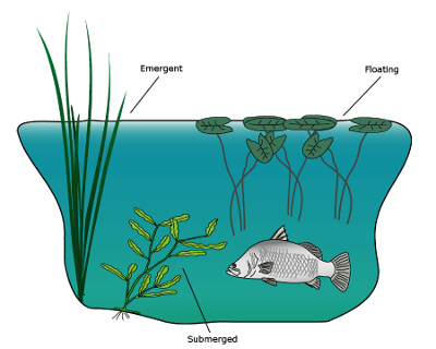
Riparian Vegetation and Macrophyte (aquatic plant)

At each SOR site riparian zone composition and size/density was evaluated.  Zone width was measured; percentage bare vegetation and floral composition were evaluated visually.  The riparian vegetation was evaluated by estimating percentage cover of the following groups: trees > 30 m, trees 10-30 m, trees < 10 m, woody shrubs > 2 m, woody shrubs < 2 m, vines, rushes and sedges, herbs and forbs, grasses, tree ferns, mosses, and palms.  Means, standard errors, max, and min values for the province were calculated from this data.   

Macrophyte composition was evaluated similarly, with visual estimation of three macrophyte categories: submerged, floating, and emergent.  These were summed to generate a total percentage cover for each site.  Means, standard errors, max, and min values for the province were calculated from this data.

Bank Shape and Slope

At each SOR site bank shape and slope were assessed visually.  For both bank slope and shape, all categories which were present were ranked in terms of their dominance (i.e. prevalence) at the site.  Bank slope categories varied in gradient.  Bank shape categories varied in structure and ecological importance.  Percentages of presence, dominance, and non-dominance were calculated from the data.

Hydrology

Modelled pre-water resource development (“natural”) daily flows between 01/01/1922 and 31/12/1995 were used as the base data for these analyses.  The Integrated Quantity-Quality Model (IQQM), developed by the Department of Land and Water Conservation (DLWC), was used as the source of the flow data.  Flow data was then analysed using the Time series analysis module[21] of the eWater River Analysis Package (RAP).

Base flow and flood flow

Base flow is considered here to be the fraction of all flow that occurs in the absence of run-off due to rainfall events. The base flow component is calculated using the methods of Grayson et al., (1996). Base Flow Index was calculated for each gauge as the ratio of total base flow to total flow for the entire reporting period, and Flood Flow Index as the ratio of non-base flow to total flow for the entire period. The average value and maximum and minimum values for the province were calculated based on all gauges.

Rise and fall of the hydrograph

The rate of rise/fall was calculated as the change in discharge for each event divided by the duration of the event. These were then averaged across all events for each gauge. The single greatest rate for each gauge was also recorded. These values were then divided by the mean daily flow across the entire record for each gauge to standardise the gauges. Note: this standardisation will be replaced with an improved method using proportional changes when RAP is updated. The average value and maximum and minimum values for the province were calculated based on all gauges.

No Flow Spells

The occurrence and characteristics of no flow (dry) spells were evaluated for each gauge and a number of summary values collected.  These were averaged across sites and used to produce annual values.  The variables collected were: frequency of no flow spells, proportion of time with no flow, longest no flow spell (days), mean duration of no flow spells (days), mean period between no flow spells (days), longest period between no flow spells (days).  The threshold for definition of a no flow spell was 2 Ml day^-2 due to constraints of the IQQM models. 

Wet and dry seasons

For each gauge the average across the entire record of monthly total flow for each month was calculated as a proportion of the sum across all 12 months. The average value and maximum and minimum values for the province were calculated based on all gauges.

Magnitude of spates

The magnitude of extreme events (spates) in each province was defined by considering the magnitude of the 10th percentile of daily flows over the reporting period. This is the value that is exceeded by only 10 percent of days in the record and was arbitrarily chosen to represent extreme high flow events. Because the magnitude is partly a function of catchment area, daily flows were standardised by dividing by catchment area for this calculation and the 10th percentile of daily flows is thus presented as Ml km² day^-1. The average, maximum and minimum values across all gauges in the province were calculated to represent the province.  Spate frequency and duration in each province was defined by considering the magnitude of the 10 th percentile of daily flows over the reporting period. This is the value that is exceeded by only 10 percent of days in the record and was arbitrarily chosen to represent extreme high flow events. The average number of spates and duration of spates per year and the average number of spates per year occurring in each of the wet and dry seasons were calculated. The average, standard error, maximum and minimum values across all gauges in the province were calculated to represent the province.

Frequency and duration of spates

The frequency and duration of extreme events (spates) in each province was defined by considering the magnitude of the 10th percentile of daily flows over the reporting period. This is the value that is exceeded by only 10 percent of days in the record and was arbitrarily chosen to represent extreme high flow events. The average number of spates and duration of spates per year and the average number of spates per year occurring in each of the wet and dry seasons were calculated. The average, standard error, maximum and minimum values across all gauges in the province were calculated to represent the province.

Water Quality

Turbidity

Turbidity (Nephelometric Turbidity Units (NTU)) was measured in the field by means of a meter at ABMAP reference sites throughout Queensland whenever macroinvertebrate samples were collected. Mean site values were calculated for sites sampled on multiple occasions and from these data, mean, maximum and minimum values were calculated for each province.

Photic Zone Depth

Light penetration on the water column has been investigated in some Queensland rivers[4][3]. Photosynthetically active radiation (400 – 700 nm) was measured as a function of depth using an underwater quantum sensor. Extinction coefficients (Kd) were calculated using a linear regression of the natural log of the irradiance at depth divided by the surface irradiance versus depth. Photic zone depth was determined as the depth at which irradiance equalled 1% of surface irradiance.

Benthic Metabolism

Open-bottom, dome-shaped Perspex chambers were used to measure benthic metabolism (diameter = 29.5 cm, height = 35 cm) and were sealed by pushing at least 5 cm into the substrate. Chambers have a central port for an oxygen sensor and side ports for a recirculating pump. The oxygen sensor was calibrated in the field immediately prior to deployment. Thick (0.1mm) membranes were used to minimize drift[5]. Dissolved oxygen within each chamber was monitored electronically at 10-minute intervals by a data logger over at least 24 hours. After the data were downloaded from the logger, a series of computer subroutines were used to convert the information into units of carbon. This was done by assuming both a photosynthetic quotient of one[17][2] and 1 mg O2= 0.375 mg C. Further details of sampling methods can be found in Bunn et al. (1999) and Bunn and Davies (2000).

Different aspects of benthic metabolism were calculated by comparing the rate of O₂ change in the chambers at different times of the day. These are the daily respiration (R; taking the night time respiration rate and assuming this rate occurs over 24h), gross primary productivity (GPP; the daily O₂ production by photosynthesis which comprises the measured daylight production rate plus the O₂ simultaneously consumed by respiration during daylight, calculated using the night time respiration rate) and the P/R ratio (GPP divided by R24). If a system has P/R > 1, it is a net producer of organic carbon i.e. accruing biomass and termed autotrophic. If P/R = 1 the system is in steady state and, if P/R < 1 the system is a net consumer of organic carbon or heterotrophic.

Other Climate and Terrain Attributes

Introduction

A national stream and catchment database has been developed at the Centre for Resource and Environmental Studies (CRES) at the Australian National University[28]. This database attributes every stream segment (i.e. the section of stream between tributary junctions) with a number of environmental variables characterising landscape scale controls on riverine ecosystem patterns and processes. Queensland Department of Natural Resources and Mine (DNRM) requested CRES compile a statistical profile and maps of selected variables from this database for the Queensland freshwater biogeographical provinces to assist DNRM with the development of conceptual models of aquatic ecosystem function. A report was produced to provide a brief description of the work undertaken, the derivation of the landscape variables and information to assist interpretation[29].

Methods

A statistical summary of each variable (Table 1) for each province was computed using grid overlay functions within the GIS software, ArcInfo[6]. Summary tables were provided in Microsoft Excel spreadsheet format. Quantitative variables were mapped using a continuous colour ramp and a linear stretch of values between the lesser of the mean plus or minus two standard deviations and the data extremes. Province profiles for categorical variables (flatness class) were derived in the form of a contingency table.

Freshwater Biogeographical Provinces

A digital coverage of the biogeographical province boundaries was prepared using a shape file of catchment boundaries and a map showing freshwater provinces and their member catchments provided by the Aquatic Ecosystem Health Unit of DNRM. The province coverage was gridded at a resolution of 9 seconds of latitude and longitude to match environmental variables.

Variable Definition and Derivation

Statistical profiles and maps were compiled from attribute grids with a spatial resolution of 9 seconds of latitude and longitude, or approximately 250m. Most of the topographic and climatic parameters were computed from version 3 of the national 9 second Digital Elevation Model (DEM).  Some background information on the attributes and potential sources of uncertainty in the data can be found here. It incorporates over 22,000 sink or depression points identified from 1:100,000 scale topographic maps. The stream network used to compute those variables attributed to individual stream segments (relief ratio, slope and annual mean run-off) was delineated from the surface flow pathways defined by the DEM using new methods of drainage analysis[28].

Variable	Code	Summary Object	Units	Description
Terrain parameters
Relief Ratio	reliefratio	stream segment	dimensionless	R = h / L where h = difference in elevation between the highest point on the catchment divide and segment pour-point L = maximum length of the catchment[10]
Stream segment slope	strslope	stream segment	%	S = h Elevation difference between the highest point on the segment and the segment pour-point divided by the segment length.
Flatness Index class	vbfclass	grid cell	dimensionless	Derived from multi-resolution Valley Bottom Flatness (mrVBF) and Ridge Top Flatness Indices (mrRTF)[8]
Climate parameters
Mean annual temperature	mat	grd cell	°C	The mean of all the long-term weekly mean temperatures. Each weekly mean temperature is the mean of that week's mean maximum and minimum temperatures
Highest weekly mean maximum temperature	maxt	grid cell	°C	The highest temperature of the long-term mean weekly maximum temperatures.
Lowest weekly mean minimum temperature	mint	grid cell	°C	The lowest temperature of the long-term mean weekly minimum temperatures.
Ratio hottest weekly maximum to coldest weekly minimum	maxt-mint	grid cell	dimensionless	Ratio of 5 and 6 above
Annual mean precipitation	tap	grid cell	mm	Total sum of long-term mean monthly precipitation
Driest quarter precipitation	pdq	grid cell	mm	Total sum of weekly long-term mean precipitation of the driest 13 week period
Rainfall erosivity	erosvty	grid cell	MJ mm ha-1 hr-1 yr-1	Annual mean sum of individual storm erosion index values, EI30, where E is the total storm kinetic energy and I30 is the maximum 30-min rainfall intensity
Annual mean “run-off”	annmeanrunoff	stream segment	mm	Annual mean catchment soil water surplus for the period 1968 to 1998 divided by catchment area

---

References

1. ^ Allen, GR, Midgley, SH & Allen, M (2002), Field guide to the freshwater fishes of Australia, Western Australian Museum, Perth.
2. ^ Bender, M, Grande, K, Johnson, K, Marra, J, Williams, PJL, Sieburth, J, Pilson, M, Langdon, C, Hitchcock, G, Orchardo, J, Hunt, C, Donaghay, P & Heinemann, K (1987), 'A comparison of four methods for determining planktonic community production', Limnology and Oceanography, vol. 32, pp. 1085-1098.
3. ^ Department of Environment and Resource Management (2010a), Waterhole persistence and productivity in two rivers in northern Queensland: TRaCK research highlights, Queensland Government, Brisbane.
4. ^ Department of Environment and Resource Management (2010b), Refugial waterholes project: research highlights, Queensland Government, Brisbane.
5. ^ Dudley, TL, D'Antonio, CM & Cooper, SD (1990), 'Mechanisms and consequences of interspecific competition between two stream insects', Journal of Animal Ecology, vol. 59, pp. 849-866, British Ecological Society.
6. ^ ESRI (2004), ArcGIS 9.0.
7. ^ Gallant, J, personal communication (16 April 2004).
8. ^ a b Gallant, JC & Dowling, TI (2003), 'A multiresolution index of valley bottom flatness for mapping depositional areas', Water Resources Research. [online], vol. 39, no. 12. Available at: https://agupubs.onlinelibrary.wiley.com/doi/10.1029/2002WR001426.
9. ^ GEODATA TOPO-250K User Guide (1992), Australian Survey and Land Information Group, Canberra.
10. ^ a b c d Gordon, ND, McMahon, TA, Finlayson, BL, Gippel, CJ & Nathan, RJ (2004), Stream hydrology: an introduction for ecologists, John Wiley and Sons, Chicester.
11. ^ Hutchinson, MF (1998), 'Interpolation of rainfall data with thin-plate smoothing splines II: Analysis of topographic dependence', Journal of Geographic Information and Decision Analysis, vol. 2, pp. 168-185, Geography Department - University of Western Ontario: London, CA.
12. ^ a b Hutchinson, MF, Houlder, DJ, Nix, HA & and Mcmahon, JP (2000), ANUCLIM Users Guide Version 5.1., Australian National University, Centre for Resource and Environmental Studies, Canberra.
13. ^ Hutchinson, MF, Nix, HA & McTaggart, C (2004), GROWEST Version 2.0, Australian National University, Centre for Resource and Environmental Studies, Canberra.
14. ^ Jeffrey, SJ, Carter, JO, Moodie, KB & Beswick, AR (2001), 'Using spatial interpolation to construct a comprehensive archive of Australian climate data.', Environmental Modelling & Software, vol. 16, no. 4, pp. 309-330, Elsevier.
15. ^ Kay, WR, Halse, SA, Scanlon, MD & Smith, MJ (2001), 'Distribution and environmental tolerances of aquatic macroinvertebrate families in the agricultural zone of southwestern Australia', Journal of the North American Benthological Society, vol. 20, pp. 189-199, The Society for Freshwater Science.
16. ^ Kesteven, J, Landsberg, J & Australia, U (2004), 'Developing a national forest productivity model', Technical Report, vol. 23, p. 104, National Carbon Accounting System, ed. A G Office.
17. ^ Lambert, W (1984), 'The measurement of respiration', A Manual on Methods for the Assessment of Secondary Productivity in Fresh Waters.  Second Edition, pp. 413-468, Blackwell Scientific, Oxford, eds. J A Downing & F H Rigler.
18. ^ Leggett, R (1993), Distributional records of freshwater fish collected within Queensland by Ray Leggett 1950-1993, Ray Leggett, Caboolture.
19. ^ Lu, H, Gallant, J, Prosser, IP, Moran, C & Priestley, G (2001), 'Prediction of sheet and rill erosion over the Australian continent, incorporating monthly soil loss distribution', CSIRO Land and Water Technical Report, vol. 13, CSIRO Land and Water.
20. ^ a b Lu, H & Yu, B (2002), 'Spatial and seasonal distribution of rainfall erosivity in Australia: Rainfall erosivity in Australia', Australian Journal of Soil Research, vol. 40, pp. 887-901, CSIRO.
21. ^ Marsh, N (2004), Time Series Analysis Module: River Analysis Package. [online], Cooperative Research Centre for Catchment Hydrology, Monash University, Melbourne, Australia. Available at: https://wiki.ewater.org.au/display/SD50/River+Analysis+Package#RiverAnalysisPackage-TimeSeriesAnalysismodule.
22. ^ McDowall, RM (1996), Freshwater Fishes of South-eastern Australia, Reed Books, Chatsworth, NSW, Australia.
23. ^ Moffatt, DB & Voller, JK (2002), Fish and fish habitats of the Queensland Murray-Darling Basin, Department of Primary Industries Queensland.
24. ^ Nix, HA (1981), 'Simplified simulation models based on specified minimum data sets: The CROPEVAL concept', Application of remote sensing to agricultural production forecasting, pp. 151-169, Commission of the European Communities, Luxembourg, ed. A Berg.
25. ^ a b Nix, HA (1986), 'Biogeographic analysis of Australian elapid snakes', Atlas of Elapid Snakes of Australia.  Australian Flora and Fauna Series No. 7, pp. 4-15, Australian Government Publishing Service, Canberra, Australia, ed. R Longmore.
26. ^ Pusey, B, Kennard, M & Arthington, AH (2004), Freshwater fishes of north-eastern Australia, CSIRO.
27. ^ Shannon, CE (1948), 'A mathematical theory of communication', Bell System Technical Journal, vol. 27, pp. 379-423;623-656, Bell System.
28. ^ a b Stein, JL (2004), A national landscape framework for river and stream conservation developing a new stream and catchment reference system, Fourth Australian Stream Management Conference, Launceston,Tasmania.
29. ^ Stein, JL (2005), Landscape characteristics of Queensland Freshwater Biogeographical Provinces, Centre for Resource and Environmental Studies, Australian National University.
30. ^ Tait, JTP, Choy, S & Lawson, R (2002), Bioregional frameworks for assessments of freshwater biodiversity in Australia, World Congress on Aquatic Protected Areas, Cairns, Australia.
31. ^ Thorne, CR (2004), 'Basin', Microsoft Encarta Online Encyclopedia, Microsoft.
32. ^ Vannote, RL, Minshall, GW, Cummins, KW, Sedell, JR & Cushing, CE (1980), 'The river continuum concept', Canadian Journal of Fisheries and Aquatic Sciences, vol. 37, pp. 130-137, NRC Research Press (Canadian Science Publishing).
33. ^ Wager, R (1993), 'The distribution and conservation status of Queensland freshwater fishes', Information Series, Queensland Department of Primary Industries, Brisbane.
34. ^ Wager, R & Unmack, PJ (2000), Fishes of the Lake Eyre catchment of Central Australia, Department of Primary Industries and Queensland Fisheries, Queensland, Australia.
35. ^ Zar, JH (1984), Biostatistical Analysis, 2nd ed, Prentice-Hall International Editions.

Last updated: 30 October 2019

References

Last updated: 30 October 2019 This page should be cited as: Department of Environment, Science and Innovation, Queensland (2019) Freshwater biogeographic regionalisation method, WetlandInfo website, accessed 18 March 2024. Available at: https://wetlandinfo.des.qld.gov.au/wetlands/what-are-wetlands/definitions-classification/classification-systems-background/methods/ |